
Beyond Implied Volatility
By Blu Putnam, CME Group
Published: 12 October 2018
All examples in this report are hypothetical interpretations of situations and are used for explanation purposes only. The views in this report reflect solely those of the author and not necessarily those of CME Group or its affiliated institutions. This report and the information herein should not be considered investment advice or the results of actual market experience.
We have observed in studying financial markets that 100-year floods occur quite often, maybe several every decade, so we know simple risk models can be inadequate and misleading. Many financial risk models start with a risk reading taken from the options markets – implied volatility. Implied volatility is a standard deviation-based metric and typically embeds the presumption of a bell-shaped curve. Starting with implied volatility, the risk manager or financial analyst then must work to augment the tails of the probability distribution to increase the odds of extreme events actually happening to align more closely with historical experience. After all, it is the extreme events that can do the most financial damage, so it is critical that the expected probability distribution be augmented beyond a simple standard deviation analysis to properly account for the possibilities.
Our approach and perspective is quite different. We believe that starting points matter. Starting one’s risk analysis with implied volatility introduces some hidden biases that may be surprisingly hard to overcome.
To begin with, volatility is a poor measure of risk. Many analysts like volatility because the historical standard deviation is easy to calculate and fits nicely into basic risk systems and mean-variance portfolio models. The problem is that an investor, or a financial institution for that matter, may have asymmetrical risk preferences, preferring to avoid substantive losses rather than to make large gains. That is, if avoiding large losses is the primary risk, then a symmetrical standard deviation based metric that only looks at the noise level and not the extremes is certainly not appropriate.
Another challenge is that implied volatilities are typically calculated from straightforward options pricing models that embed the heroic assumption that prices move up or down with continuous trading – that is, price breaks or price gaps are assumed never to occur. If market participants fear the possibility of price breaks, options prices will reflect this risk with a higher calculated implied volatility. But it will not be easily apparent that the implied volatility is reflecting price gap risk instead of an upward shift in the volatility regime. And, price gap risk is not the same risk as volatility regime shift risk. Depending on one’s financial exposures, one of these risks could be much more important than the other. For those managing options portfolios, for example, the risk of an abrupt price break can do considerable damage to delta hedging strategies, while a volatility regime shift represents a different risk, commonly known as “vega” risk. What one needs to create is a comprehensive view of the whole risk probability distribution providing a robust perception of risks, allowing for decidedly different risk scenarios, and not being biased toward bell-shaped curves.
To build a risk probability distribution that is not necessarily bell-shaped or even of a single mode and can capture the extremes in a robust manner, we prefer to start from a very different point of view. We start with the Bayesian prior of a very unusual distribution – in our case, a bi-modal distribution that might reflect a type of binary or two-scenario risk often associated with event risk. Then, we examine market data to see if the risks are actually more bell-shaped. While the implied volatility is one of the market metrics we examine, it does not necessarily have the primary influence it does when it is the starting point for the risk analysis.

Put another way, if we start from a prior of an extreme and unusual distribution, we know that it can exist and we have not assumed it away. Starting from a standard deviation approach, such as implied volatility, may inadvertently make it very hard to estimate when extreme and highly dangerous risk distributions are present. The math behind this observation is quite old and goes back to the Russian mathematician, Pafnuty Lvovich Chebyshev (1821 – 1894). What most people take away from Chebyshev’s Inequality Theorem is that if you know only the standard deviation you have a very good idea of the typical ranges in which values will fall the vast majority of the time. What we take away from the Inequality Theorem is that if you only know the standard deviation, you know absolutely nothing about the extremes of the distribution where the most dangerous risks reside.
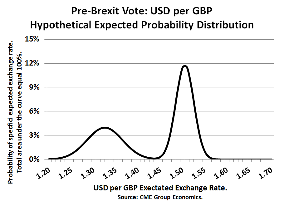
The motivation for our research was the observation that in financial markets, especially since 2016, we have and will be seeing important episodes of event risk associated with elections – UK Brexit Referendum of June 2016, U.S. Presidential election of November 2016, French and UK elections in 2017, Brazilian elections of October 2018, U.S. Congressional elections of November 2018, etc. This led us to a study of how markets cope with two strikingly different scenarios – a type of event risk. When there are two possible scenarios, then pre-event, the market is going to price the probability-weighted outcome, or the middle ground. So, post-event, when the outcome becomes known, the market immediately moves away from the middle ground to the “winning” scenario – a price break. For example, with Brexit, the “Leave” vote generated a sharp downward move in the British pound (vs USD), while a “Remain” vote would have presumably generated a sharp almost instantaneous rally in the pound – either way, the pound was no longer going to trade in the middle. Even if they are relatively rare, if one’s risk system cannot create the possibility of a bi-modal probability distribution, then price break risk and tail risk may be greatly underestimated.
From a practical perspective, starting with the prior of an abnormal, bi-modal risk probability distribution requires some creativity that might put off some risk managers. The challenge is that expected risk-return probability distributions cannot be directly observed. What we are able to do is to estimate some of their characteristics from looking at market behavior – prices, volumes, futures versus options, intra-day activity, etc.
While our research is still at the early stages, we have found a few metrics that are especially enlightening relative to the shape of the probability distribution. Our three primary metrics are: (1) the evolving pattern of put option trading volume relative to call option volume, (2) intra-day market activity, especially high/low spreads, and (3) implied volatility from options prices relative to historical volatility pattern shifts.
Studying put/call volume patterns helps us understand if one side of the market is more at the center of the current debate than the other side. For example, immediately after former Federal Reserve (Fed) Chair Ben Bernanke threw his famous “Taper Tantrum” in May 2013, he set off a debate about if and when the Fed would withdraw quantitative easing (QE) and raise interest rates. Put volume on Treasury note and bond prices soared relative to call volume as an indicator that a two-scenario situation had developed. While there is a buyer and a seller for every trade; one side thought prices would fall (yields rise) and volatility might rise very soon (buyer of puts), while the other side thought the process of exiting QE would take a long time (seller of puts).
Intra-day market dynamics help us appreciate risk in a different way. The observed high price to low price intra-day trading spread is informative in helping us assess the degree to which fat-tails might be present. Mathematically, work by Mark B. Garmin and others back in the 1970s and 1980s has shown that if one assumes a normal distribution then there is a straightforward way to estimate the standard deviation of daily returns from the intra-day high-to-low spread. Put another way, if the relationship between intra-day dynamics and the day-to-day standard deviation diverge in a significant manner, then this is strong evidence that the risk probability distribution is not normally distributed.
To ascertain the risk of price breaks we track the evolving pattern of implied volatility relative to historical volatility. While it is usual for implied volatility to exceed recent historical standard deviations, a shift in the pattern toward a much higher implied volatility may indicate that expectations for the potential of a sharp price break are building in the market. And, if a price break occurs, we often see a quick decline in the implied volatility representing a shift back to a single-mode bell-shaped distribution.
We use a probability mixture technique that is distribution independent to combine our metrics and what we find is that most of the time, bell-shaped curves are appropriate descriptions of the probability distributions. Our method does, however, occasionally generate some especially tall distributions (i.e., high kurtosis), which we classify as “complacent” and worthy of special study to see if the market may be underestimating risks. We also see on occasion some very flat distributions, not unlike the Wall Street maxim about the equity markets “climbing a wall of worry.” And, finally, on rare occasions our metrics actually support the idea of a two-scenario, event risk, bi-modal distribution. The most likely source of event risk and bi-modal distributions are highly polarized elections, when the candidates are far apart and the vote is closely contested. We classify these event risks as “known date, unknown outcome”. We also see event risk around “unknown date, unknown outcome”, which has shown up when the US-induced trade war evolves into a tit-for-tat tariff retaliation episode. This type of event risk, for example, hit soybeans, quite hard during 2018. Policy decisions taken at scheduled meeting, like a Fed interest rate decision or an OPEC oil production decision fall into the “known date, unknown outcome” category, but they almost always are associated with bell-shaped probability distributions, because the policy makers go out of their way to telegraph the decision ahead of time, reflected in the fact that our metrics pick up no unusual risks.