All examples in this report are hypothetical interpretations of situations and are used for explanation purposes only. The views in this report reflect solely those of the author and not necessarily those of CME Group or its affiliated institutions. This report and the information herein should not be considered investment advice or the results of actual market experience.

Whether we are talking about an election outcome, a fiscal or monetary change of policy direction, the trade war, or even the possibility of a drought in the farm belt, we have event risk. And, event risk typically involves two divergent scenarios. If the two scenarios are far enough apart from each other, then event risk has the potential to create a risk-return probability distribution that may look more like bi-modal distribution than the common single-mode bell-shaped curve. These are rare distributions, more like the two-humped Bactrian camel of Mongolia than the common single-hump Dromedary camel of the Middle East.

Event risk market environments come with a much greater likelihood of price gaps as well as the potential for a shift in the volatility regime than one would typically capture in a risk model anchored by implied volatilities from option prices or, indeed, any risk model based on standard deviations as the primary metric representing risk. Therefore, it is incredibly important to recognize the market characteristics that warn of event risk, and one needs to have a risk management process that can accommodate these rare and unusual bi-modal distributions.

I. Difficulties in Capturing Event Risk with Implied Volatility from Options Prices

Starting from a standard deviation approach, such as implied volatility, may inadvertently make it very hard to estimate when extreme and highly dangerous risk distributions are present. The math behind this observation is quite old and goes back to the Russian mathematician, Pafnuty Lvovich Chebyshev (1821 – 1894). What most people take away from Chebyshev’s Inequality Theorem is that if you know only the standard deviation you have a very good idea of the typical ranges in which values will fall most of the time. What we take away from the Inequality Theorem is that if you only know the standard deviation, you know absolutely nothing about the extremes of the distribution where the most dangerous risks reside.

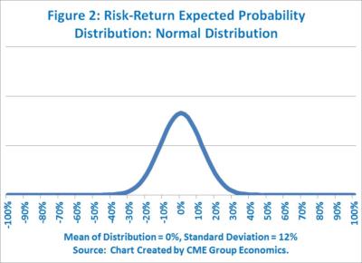
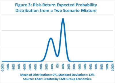
As an example, the two probability distributions in Figures 2 and 3 have the same mean and standard deviation, but they indicate very different risk management challenges. Figure 2 is a normal, single-mode, bell-shaped distribution, while Figure 3 is bi-modal distribution which was created by mixing two normal distributions with highly divergent means and different standard deviations for each scenario. We want to highlight two risk management challenges of note when event risk is present to the degree that it would be reflected in a bi-modal risk-return probability distribution.

The first risk we want to examine is that of a price gap when the outcome of the event risk becomes known. If you take the Brexit case, at the time of the referendum, one can get a feel for the price gap risk. At the time of the referendum back in June 2016, it was widely believed that a “Leave” vote would result in an abrupt weakening of the British pound, and that a “Remain” vote would create an instantaneous relief rally, raising the value of the pound. As the “Leave” outcome became clear on the night of the referendum, the pound, indeed, had a sharp 7% dive versus the US dollar. Prior to the event, the market was pricing the probability weighted average of two divergent scenarios, and once the outcome was known, the market immediately moved to a single-mode distribution centered on the “winning” outcome.

In our analysis, we want to try to identify the conditions which might cause price gap risk and to measure the intensity of the potential divergence in the scenarios. The importance of studying the probability of price gap risk is that basic options pricing models, such as Black-Scholes-Merton and straightforward options hedging strategies explicitly rule out any possibility of price gaps. And a large price gap (i.e., a price discontinuity in the language of Black-Scholes-Merton) can effectively destroy a standard delta hedging approach to managing options risk.

The second risk of note coming from event risk is the possibility of a shift in the volatility regime. As in the case of price gap risk, the basic Black-Scholes-Merton options pricing models assume that a volatility regime shift cannot occur. Of course, during the pre-event risk phase, there may be one volatility regime, followed by a shift to new volatility regime, possibly higher or lower, after the outcome is known. This is known as vega risk in the options world and has been well studied, especially since the stock market crash of October 1987 alerted one and all to its implications for options risk management.

Observing price gap risk from implied volatilities is very tricky. When the date of the event risk is known, such as in the case of a referendum or election, then one can examine options with similar strikes that expire before the known event risk date and afterwards. Differences in implied volatility between the two expiry dates can be attributed, with care to consider other factors that may be operating simultaneously, as a metric indicating the existence of price gap risk.

Comparing options with different expiry dates that bracket the known event risk date, however, breaks down if the event risk date is unknown. [See “The Changing Nature of Event Risk” in AMIA Issue #117, January 2019.] For example, during 2017 in the US, there was an active discussion of a large cut in corporate taxes which would clearly benefit equities. The problem was that one did not know if or when the corporate tax cut would be passed into law. Indeed, during the spring of 2017, when the debate over repealing the health care legislation known as the Affordable Care Act was at its most intense, markets participants appeared to lower the probability of a tax cut passing Congress. Later in the year, however, it became increasingly clear that a large corporate tax cut would be passed and signed by the President into law. This is an example of event risk without a specific decision date. One could argue that the trade war had this type of characteristic. Despite the US setting some short-term deadlines, one never really knew if or when a deal would be agreed. The Brexit negotiations have some of this flavor. While there is a specific end-date to the divorce negotiations, March 29, 2019, there is also the possibility of an extension.

To summarize this discussion, let’s examine the type of market expectations captured by a typical bell-shaped curve. With a bell-shaped risk-return probability distribution, one is essentially saying that there is a consensus view around the expected return with incrementally different possibilities of lower probability creating the bell-shaped risk distribution. While the market may shift in increments to a new consensus based on new information, the expected mean shifts are continuous and do not constitute price gap risk, and the expected volatility remains more or less the same. In the case of a bi-modal risk-return probability distribution, there is the possibility of an abrupt shift in the expected mean (price gap risk) and a shift to a new volatility regime.

II. A practical approach to event risk probability distribution analysis

While our research is still at the early stages, we have found a few metrics that are especially enlightening relative to the shape of the probability distribution. Our three primary metrics are: (1) the evolving pattern of put option trading volume relative to call option volume, (2) intra-day market activity, especially high/low spreads, and (3) implied volatility from options prices relative to historical volatility.

Studying put/call volume patterns helps us understand if one side of the market is more at the center of the current debate than the other side.

Intra-day market dynamics help us appreciate risk in a different way. The observed high price to low price intra-day trading spread is informative in helping us assess the degree to which fat-tails might be present. If the relationship between intra-day dynamics and the day-to-day standard deviation diverge in a significant manner, then this is strong evidence that the risk probability distribution is not normally distributed. To inform us about the risk of price breaks we track the evolving pattern of implied volatility relative to historical volatility. While it is usual for implied volatility to exceed recent historical standard deviations, a shift in the pattern toward a much higher implied volatility may indicate that expectations for the potential of a sharp price break are building in the market. And, if a price break occurs, scenarios resolve one way or the other, so we often see a quick decline in the implied volatility representing a shift back to a single-mode bell-shaped distribution.

To gather all our risk information and create a probability distribution, we use a probability mixture technique that is distribution independent – that is, it is not constrained to take on a given specified shape. Most of the time, bell-shaped curves are appropriate descriptions of the probability distributions – balanced risk distributions. Our method does, however, occasionally generate some especially tall distributions (i.e., relatively lower volatility), which we classify as “complacent” and worthy of special study to see if the market may be underestimating risks. We also see on occasion some very flat distributions, not unlike the Wall Street maxim about the equity markets “climbing a wall of worry” which we call “anxious” risk distributions. And, finally, on rare occasions our metrics support the idea of a two-scenario, event risk, bi-modal distribution. Looking at a wide variety of markets, we seem to find event risk being reflected in a bi-modal distribution only about 2% to 3% of the time, with balance risks dominating at about 70% or so, and the “complacent” or “anxious” distributions making up the difference.