Introduction

We’ve long thought that regimes – specific market environments characterised by distinct macroeconomic, financial and geopolitical conditions over a set time period – offer a useful perspective on performance and risk. 

In this paper, we construct a simple model that characterises markets by their similarity or difference when compared to historical periods. Our aim is to provide a point-in-time metric for timing investments by proposing a systematic approach to regime selection (a ‘Regime Model’). 

To test for real-world applicability, we apply our Regime Model to six popular long-short equity factors. We go long a factor if the historical return after observing the regime at the investment date is positive, and short otherwise. 

Our research documents a positive relation between the returns and similarity. Indeed, the least similar historical dates do the worst in terms of performance. The alpha of being long the most similar and short the least similar is a statistically significant three standard deviations from zero. 

The Regime Model methodology

The user of our Regime Model needs to specify a set of economic variables. In this paper, we consider seven variables, transform each of them to look at annual changes and compute a z-score. Then, variable by variable, we investigate the past and identify regimes that are similar.¹ Looking at every historical date, we aggregate the distances at each date across our seven variables, to create an aggregated similarity score (the ‘Global Score’). Those historical dates with the smallest aggregate distances are our definition of similar regimes. Once we have established similar dates in the past for a particular asset, we look at subsequent returns. With the historical regimes established, we can apply this method to any asset class. 

Our Regime Model has several advantages. First, the method is systematic (the regime classifications are automatic). Second, the method can be applied to a much larger set of economic variables. Third, our method is simple, relying only on z-scores. 

That said, in any systematic model, choices need to be made. Here, the economic state variables need to be chosen. Second, there is a choice as to how to represent each variable (e.g., what horizon for rate of change?). Third, we need to set the degree of similarity. Fourth, we need to decide the length of the observation period after the similar historical regime. Finally, how should we weight the economic variables?

Economic state variables

We use the seven economic state variables detailed in Exhibit 1:²

Exhibit 1. Economic state variables and sources
 

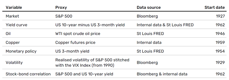
For each variable, we take a 12-month change and then normalise it by computing the z-score over a rolling 10 years, capped to be within minus three and three.³ Next, we compute an adjustment similar to a z-score, whereby we divide the one-year difference by the standard deviation of the rolling one-year differences, computed over 10 years. We finish by winsorizing at three to remove outliers, thereby creating the transformed economic state variables.

We now apply our distance-based similarity metric. Each month we iteratively compute the Euclidean distance – the distance ‘as the crow flies’ – between each historical month and the month in question.⁴ We are then able to aggregate across our variables, to obtain one Global Score.⁵ Historical months with smaller similarity scores are the most similar to today.

Similarity in action: the Global Financial Crisis (GFC)

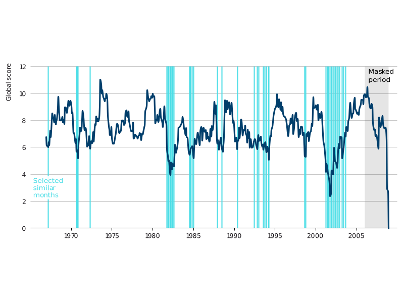
To illustrate how our Regime Model works, we can apply it to the GFC. For specific months, we examine the full history and pick the 15% most similar months (i.e., the 15% of months with the lowest Global Score). We exclude the last three years (36 observations), as this helps us to avoid loading up on momentum.

Referring to the GFC, Exhibit 2 considers the Global Score as of January 2009. The most similar dates have the lowest values and include all observed recessions. Our trading strategy would take a long position in an asset in February 2009 that exhibits positive returns after historically similar regimes. 

Exhibit 2. Historical similarity to January 2009 during the GFC

Assessing the predictive power of the Regime Model 

We illustrate the efficacy of our methodology on six long-short stock factors: using the Fama-French five research factors (Market, Size, Value, Profitability and Investment) plus the 12-month Momentum factor.

Exhibit 3 shows the aggregate performance of investing in the six factors (on an equally weighted basis) using the 20% most similar historical dates (quintile one). We are long a factor if the average of returns after the most similar dates was positive, and short if it was negative. We repeat this exercise for the other quintiles, and so quintile five utilises the 20% most dissimilar dates. On the left-hand chart in Exhibit 3, we have included the performance of quintile one and quintile five (of the five quintiles, quintile one performs best and quintile five performs worst). We also include a representative long-only model (LO model) which serves as a proxy for a traditional long-only portfolio. While you can see that the LO model performs slightly better than quintile one over time, it brings with it significantly worse drawdowns during crisis periods. 

Exhibit 3: Assessing the predictability using six long-short stock factors⁶
 

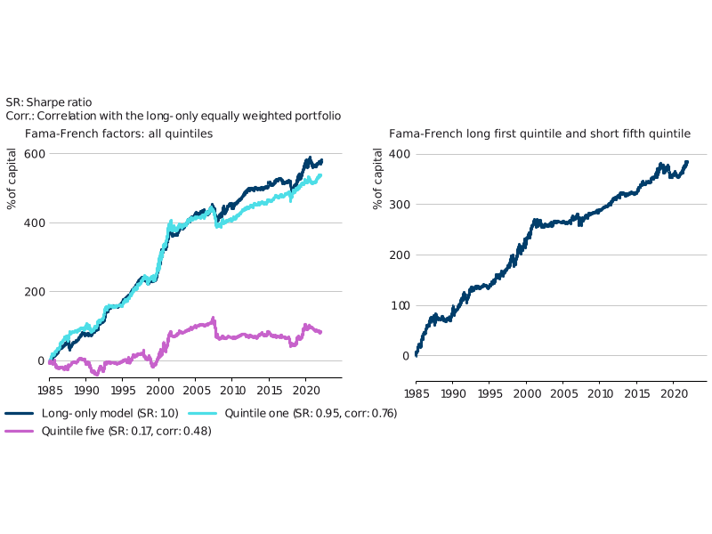
As factors tend to have positive returns on average, we can create a less correlated ‘difference’ portfolio by going long the quintile-one portfolio and short the quintile-five portfolio (Exhibit 3, right-hand chart). This portfolio has an impressive 0.82 Sharpe ratio, while only being 0.37 correlated to the long-only portfolio. The alpha is significant, being three standard errors from zero.

Conclusion: Diversification via multiple variables 

Our Regime Model is a systematic method to identify economic regimes, which assesses the similarity of any month to the history of a selection of economic time series. The user specifies the economic time series as well as the tolerance for similarity and can specify many economic variables to achieve diversification.

We use our method to actively time six well-known factors. We aggregate all factors and find there is important information in the similarity. The strategy based on the most similar periods does well. We also find that in the anti-regime months (the most dissimilar), the performance is poor.

There are many possible research enhancements. We equally weight the economic variables, rather than a dynamic weighting based on predictive performance. Further, we assess similarity to particular months. If the investment horizon is longer than a month, it might be reasonable to look at similarity relative to a quarter or longer. These and related ideas are for future research into economic regimes.
 

Important information - Disclaimer.

¹ Our measure of similarity is the squared distance of today’s value to each historical observation. For example, if the z-score today is 2.5, we look at historically similar times where the z-score is close to 2.5. For a historical date value of exactly 2.5, the squared distance would be zero.

²  These were selected after a systematic process to establish which variables were the most important driver of equity returns. All are financial variables that embed macroeconomic information.

³  We use monthly data so that we can extend our history as far back as possible. For the correlation series we use a rolling three-year metric. We run this on daily data before converting to monthly.

⁴  This calculation must be done for every historical month. For example, if the variable has a score of 2.5 in December 2024, we calculate the distance between each historical month and 2.5.

⁵  The Euclidean distance, d, is defined by: d_Ti=√(∑_v^V(x_iv-x_Tv )^2 ). On a selected month T, for every historical month i, we calculate a sum of squares of the V transformed variables. We do so by computing the absolute difference between the value of each variable at month i, xiv, and the value of each variable at month T, xT v. We sum across variables before taking the square root, to give us our similarity score, dT i, for every month up to month T.

⁶  The performance of investing in the six long-short stock factors. For the quintile one portfolio, the direction taking in a factor is based on returns subsequent to the 20% most similar historical dates. The quintile five portfolio utilises the 20% most dissimilar returns. The long-only portfolio is long all six factors throughout. Performance is shown for 1985-2024. Input data starts well before 1985 to allow for rolling-window calibrations.